
sheelamohanachandran - Fotolia
Oracle E-Business Suite manufacturing and supply chain management
Find out what the Oracle E-Business software suite can do for manufacturing supply chain management (SCM). Learn supply chain planning and forecasting strategies for Oracle SCM software.
Successful supply chain management (SCM) starts with strong supply chain planning. In this book chapter excerpt, find out what the Oracle E-Business software suite can do for your manufacturing SCM strategy.
Discover material and capacity planning techniques and learn supply chain forecasting tips to use with Oracle SCM software.
The Oracle Applications suite currently offers two products for material and capacity planning in a manufacturing or distribution environment: Master Scheduling/MRP and Advanced Supply Chain Planning.
Master Scheduling/MRP offers single-organization, unconstrained planning of material and resources. We'll use the term MRP to refer to this planning tool. Advanced Supply Chain Planning (ASCP) is the next-generation planning tool; it offers multi-organization planning and the option of constraint-based and optimized plans.
Copyright information

The following book excerpt is taken from Chapter 8 of the McGraw-Hill Osborne Media book, "Oracle E-Business Suite Manufacturing & Supply Chain Management," by Bastin Gerald, Nigel King and Dan Natchek.
Click to download the full chapter.
This chapter describes the basic logic common to both planning methods and details the common setup needed by both methods. Subsequent chapters describe the unique characteristics of MRP and ASCP.
Note
In past releases, Oracle sold a product called Supply Chain Planning, which provided the capability of planning across a supply chain, but without the constraints, optimization, and variable granularity of the Advanced Supply Chain product. With Release 11i, this is no longer sold as a separate product, so it will not be explicitly covered in this book. However, much of material describing Advanced Supply Chain planning applies to the older supply chain planning; notable exceptions are the constraint and optimization capabilities of ASCP and the treatment of sourcing rules, which are described in Chapter 11.
Basic planning logic
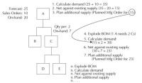
The basic logic of both MRP and ASCP is time tested and well documented in numerous sources. Though not a comprehensive discussion of basic MRP logic, what follows is a brief overview of the process. The process is illustrated in Figure 8-1. It involves the recognition of demand or requirements, the netting of those requirements against available and scheduled quantities, and the generation of recommendations to meet those requirements. In a manufacturing environment, the process proceeds top-down through the bill of material, so that recommendations at one level form the basis of the requirements on the next level of components, and so on.
Recognition of demand
Demand initially starts as a statement of what a company expects to sell or ship. This type of demand represents what you know or think you are likely to sell outside your company and is traditionally called independent demand because it is to some extent outside of your control. In a manufacturing business, the independent demand for your finished goods determines the demand on the component parts; this is called dependent demand, since it depends on, and can be calculated from, your bills of material.
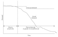
Independent demand is typically some combination of forecast and actual (Sales Order) demand. Depending on the stocking strategy you employ for a particular product, the mix of forecast and actual demand will vary; in a make-to-stock strategy, you will rely heavily, perhaps exclusively, on forecast demand. In a make-to-order strategy, you will rely heavily on actual sales orders. Furthermore, the ratio of forecast to actual will likely vary over the time horizon, as shown in Figure 8-2 -- in the near term, you might rely most heavily on actual demand, while using forecast demand at the midora- and long-range points of the time line.
Oracle Applications allow you to have alternate forecast scenarios, so the forecasts you want to use to plan, as well as the actual demand you want to recognize, are stated in a Master Demand Schedule (MDS). The MDS is discussed in more detail, in the "Master Scheduling" section.
Dependent demand is demand calculated from the explosion of your bill of material. An important premise of MRP planning is that you should calculate, not forecast, dependent demand. For example, one automobile requires four tires; if you forecast or sell one auto, you know you will need four tires to build it. There's no point in forecasting tires; you can calculate the requirements from the bill of material.
Because they represent an attempt to predict the future, forecasts are notoriously inaccurate; forecasting what you can calculate can only compound problems.
It is possible that one item can have both independent and dependent demand. If you were to sell tires as service parts, in addition to including them on a manufactured auto, you would want to forecast the independent portion of the demand on tires while calculating the dependent demand.
Gross-to-net calculation
Once the demand is known, the next step is to determine how much of that demand can be satisfied from existing stock or existing orders. It's simple arithmetic; if you have gross requirements (total demand) for 100 units of a product, and you have 25 on hand, the net requirements are 75.
Time-phasing makes this arithmetic a little more interesting. If that same demand were spread out over four weeks (25 per week), your 25 on-hand would satisfy the first week's demand. If you had an existing order (e.g., a manufacturing order) to build 25 more in week 3, the system would expect you to reschedule that order to satisfy the demand in week 2 and would then see net requirements for 25 each in weeks 3 and 4.
Recommendations
In the scenario described earlier, the planning process would recommend that you reschedule the existing order from week 3 to week 2 and would recommend that you create new orders to satisfy the demand in weeks 3 and 4.
In this process, planning will respect any order modifiers you've attached to the item, such as minimum or maximum lot sizes. It will look at any anticipated shrinkage factors you've associated with the product and inflate the planned orders to compensate. And it will respect time fences to allow you to stabilize your production or procurement schedules in the short term. It is the application of all these factors that makes planning beyond the scope of paper and pencil for all but the simplest scenarios. Order modifiers, shrinkage, and time fences are described later in this chapter.
Bill of material explosion
In a manufacturing environment, once the top-level demands are known, the component demands are calculated based on the explosion of the bill of material. The component demand (plus any independent demand for the component) constitutes the gross requirements at the next level. The planning process then continues to calculate net requirements and plan orders at each level in the bill of material.
Planning cycles
You can use Oracle's planning products in numerous ways to generate distribution plans, master schedules, and manufacturing (MRP) plans for your enterprise. The possibilities are almost endless, but we'll discuss two typical examples here.
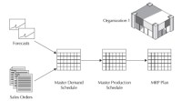
Figure 8-3 shows the traditional planning cycle. In this cycle, you create forecasts and book sales orders, load the selected forecasts and orders into a Master Demand Schedule, use the MDS as input to planning a Master Production Schedule, and submit that MPS to MRP. This cycle separates master scheduling and MRP so that you can firm up a master schedule before submitting it to MRP. You must synchronize these plans by carefully considering the timing of the running of each plan.
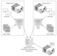
Figure 8-4 shows a holistic planning cycle; in this cycle there is only one plan that satisfies the needs of distribution planning, master scheduling, and manufacturing. You still generate forecasts, book orders, and load demand schedules, but you use one or more demand schedules from multiple organizations to generate one complete supply chain plan.
As noted earlier, numerous variants of these cycles are possible. A company that does not need to separate the Master Production Schedule from the MRP Plan can run MRP directly from the MDS. Within the supply chain plan, master schedules can be used to introduce some stability and local control into the plan. But all plans require some initial statement of demand, usually a combination of forecast and sales orders. All plans require some sort of master schedule to identify the demand that drives the plan. They will plan for effectivity date changes in your bills of material and plan for both discrete and repetitive production. These common elements are described in the following pages.
Forecasting
For most businesses, forecasts are necessary at some point in the time horizon. Even a company with a pure make-to-order strategy (if such a company exists) will probably want to use forecasts of future demand for long-range planning. Forecasting is at least as much art as science, and the art of forecasting is beyond the scope of this book. But we will describe how forecasts are represented, generated, and used within the manufacturing and supply chain planning process.
Oracle Demand Planning (described in Chapter 9) generates forecast data. In addition, the Oracle Inventory and Master Scheduling/MRP applications provide basic methods to generate forecasts from historical data, described in the section titled "Generating Forecasts from Historical Information." Forecasts can also be entered manually; imported through an open interface, described in the "Open Forecast Interface" section; or loaded via an API, described in the section titled "Forecast Entries API."
Forecast terminology and structure
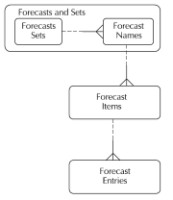
To understand the use of forecasts in planning, it is helpful to understand the terminology and data structure Oracle uses to represent forecasts. One forecast typically contains multiple items; each item has multiple entries that represent a dated demand for that item. For ease of use and to control forecast consumption, forecasts are grouped into forecast sets.
Forecasts, forecasts items, and forecast entries
Within Oracle applications, forecasts are identified by unique names. For example, you might have separate East, West, and Central forecasts, or you might have different forecast names by product line or distribution channel. You might have Optimistic and Pessimistic forecasts or simulations of various scenarios. Each such forecast is identified by a name.
Note
Give some thought to the conventions you will adopt for naming forecasts. Unlike many names in Oracle applications, forecast names (along with master schedule and plan names) are limited to 10 characters in length and cannot be changed.
A forecast will typically contain multiple item numbers, called forecast items, and each item will have multiple forecast entries, each representing the forecast demand for a particular day, week, or monthly period. (Oracle seems reluctant to use the term month unless it refers to an actual calendar month; in the context of planning, you might be using a 4-4-5 or 5-4-4 calendar, whose periods don't line up with actual calendar months.)
Your workday calendar controls the valid dates for forecast entries. Daily forecasts can be entered for working days only; weekly or period forecasts will be dated on the first day of the week or period.
Caution
If your workday calendar specifies a Quarterly Type of "Calendar months," Oracle does not currently support the use of a "Period" bucket type for forecasts.
Forecast sets
Oracle requires you to group forecasts into forecast sets, which are simply collections of forecasts. Forecast sets serve as both a convenience (you can refer to multiple forecasts by referencing their set) and a method to control forecast consumption, described in the following. This structure -- forecast sets, forecast names, forecast items, and forecast entries -- is illustrated in Figure 8-5.
Note
Forecast set names are defined in the same database table that defines forecast names, so they share the same size restrictions. In addition, forecast set names must be different from forecast names.
Generating forecasts from historical information
The Oracle Master Scheduling/MRP and Inventory Applications provide two basic methods to generate forecasts from historical data: statistical forecasting and focus forecasting. While both methods use proven algorithms, they are basic in the level of control they provide. Unlike Oracle Demand Planning, they are based strictly on the history of issue transactions (not order bookings); therefore, if you have shipped late in the past, these methods will forecast how you can ship just as late in the future! And they offer none of the outlier detection or collaborative features of Oracle Demand Planning. Nevertheless, they may meet simple requirements.
Statistical forecasts
Oracle provides basic statistical forecasting capability as part of the Inventory and Master Scheduling/MRP applications. Statistical forecasts can span multiple periods and can recognize trend and seasonality.
Focus forecasts
Focus forecasting provides a "sanity check" on the current month's forecast. Focus forecasting examines five different forecast models against past history, determines the model that would best have predicted the history, and uses that model to generate a forecast for the current period. (The process generates a "forecast" for multiple periods, but they are simply copies of the current period forecast.)
Generating forecasts
You generate a forecast by first defining a forecast rule that specifies a bucket type, a forecast method (statistical or focus), and the sources of demand. For the statistical forecast method, the forecast rule also specifies the exponential smoothing (alpha) factor, trend smoother (beta) factor, and seasonal smoothing (gamma) factor. Then, in the Generate Forecast window, you specify the following:
- Name of the forecast you want to populate.
- Forecast rule that determines the bucket, forecast method, and demand stream.
- Selection criteria to identify the items for which you want to generate a forecast. You can select all items, all items in a designated category set, items in a specific category within a category set, or an individual item.
- An overwrite option, which determines what happens to existing forecast information. All Entries deletes all existing forecasts before repopulating the forecast data. Same Source Only deletes only forecast entries that were previously generated from the same source that you are about to load. None does not delete any existing entries.
- Start date and cutoff date for the forecast information that you are about to generate.
Note
Choose the Overwrite option carefully; if you do not explicitly delete existing information through your choice of the Overwrite option, you might duplicate information already in your forecast.
Open Forecast Interface To populate forecasts using the Open Forecast Interface, you must first define your items, organizations, forecast sets, and forecast names. Then, load your forecast data into the table MRP_FORECAST_INTERFACE. Required data includes
- INVENTORY_ITEM_ID
- FORECAST_DESIGNATOR
- ORGANIZATION_ID
- FORECAST_DATE
- QUANTITY
- PROCESS_STATUS
Set the PROCESS_STATUS to 2 to designate data waiting to be processed. The Planning Manager (described later in this chapter) periodically checks the MRP_FORECAST_INTERFACE table to determine if there is any new data to be processed. If the Planning Manager detects new data, it launches the Forecast Interface Load Program. This program validates the data in the interface table and loads valid data into the specified forecast. If the load program detects an error, it sets the PROCESS_STATUS to 4 and enters a text message in the ERROR_MESSAGE column in the interface table. Use SQL*Plus, or a custom program, to view and correct invalid date in the interface.
Forecast entries API
You can use the forecast entries API to integrate with other software systems. This section describes the major steps in using this API.
1. Construct the following PL/SQL table for all the information that is associated with the forecast:
| Variable Name | Type | Meaning |
| p_forecast_entries | A PL/SQL table that contains records of type mrp_forecast_interface_ pk. mrp_forecast_ interface | These are the actual forecast entries. |
| p_forecast_designators | A PL/SQL table that contains records of type mrp_forecast_interface_ pk. rec_forecast_desg | These are the forecast designator information. |
2. Call the function mrp_forecast_interface, with the parameters that you constructed in step 1. You don't have to supply both the parameters in every case. For example, if you are inserting new forecast entries or updating existing forecast entries, you would provide all the information. On the other hand, if you are deleting all the forecast entries, you need only provide the forecast designator.
mrp_forecast_interface_pk.mrp_forecast_interface (p_forecast_entries -- INOUT PL/SQL Table for forecast entries ,p_forecast_designators -- IN PL/SQL Table for forecast designators );
3. The function returns true if the API completed successfully and false if there were failures.
Forecast consumption
In order to avoid overstating demand as actual orders are booked, forecasts are typically reduced by the amount of the sales order demand. The process is called forecast consumption. Then, when actual orders are combined with forecasts in a master schedule, the demand statement remains accurate. Forecast consumption also serves as a measurement of the forecast's accuracy -- if you've sold less than you forecast, the forecast will not be fully consumed; if you've sold too much, the result will be reflected as overconsumption at the forecast set level.
Forecast consumption is one of the functions of the Planning Manager, described later in this chapter. At its simplest, forecast consumption reduces a forecast demand by the amount of the actual sales order demand in that period. The remaining forecast quantity is referred to as the current forecast; the original forecast quantity remains visible for comparison and analysis.
The first rule of forecasting is that the forecast will be wrong. It is highly unlikely that a customer order will exactly match your forecast quantities (although supply chain collaboration might help ameliorate this problem). So, to make the process yield usable results, a number of factors influence the supposedly simple process of forecast consumption.
Forward/backward days
To compensate for the discrepancy between customer orders and forecasts, you typically provide a "window" within which the forecast will be consumed. This window is expressed as a number of working days, as determined by the shop calendar. Within this window, forecast consumption will first look backward and then forward to match the forecast with the actual demand. You define this window as an attribute of each forecast set.
Consider this example:
| Days | 1 | 2 | 3 | 4 | 5 | 6 | 7 | 8 | 9 | 10 | 11 | 12 | 13 | 14 | 15 | 16 | 17 | 18 | 19 | 20 | |||||
| Forecast | 5 | 5 | 5 | 5 | 5 | 5 | 5 | 5 | 5 | 5 | 5 | 5 | 5 | 5 | 5 | ||||||||||
| Demand | 30 |
Shaded = Non-work Day
With no window for consumption, the sales order demand on day 10 would consume the entire forecast of 5 on that day and then "have no where to go." Thus, the total demand for the second week would be 50: 30 actual and 20 of the remaining, or unconsumed, forecast, as shown here:
| Days | 1 | 2 | 3 | 4 | 5 | 6 | 7 | 8 | 9 | 10 | 11 | 12 | 13 | 14 | 15 | 16 | 17 | 18 | 19 | 20 | |||||
| Forecast | 5 | 5 | 5 | 5 | 5 | 5 | 5 | 5 | 5 | 5 | 5 | 5 | 5 | 5 | 5 | ||||||||||
| Demand | 30 | ||||||||||||||||||||||||
| Unconsumed | 5 | 5 | 5 | 5 | 5 | 5 | 5 | 0 | 5 | 5 | 5 | 5 | 5 | 5 | 5 |
Daily buckets; Backward Days = 0, Forward Days = 0, Shaded = Non-work Day
With forward and backward days set to 3, the actual demand would "search" for forecast if there was not sufficient forecast quantity remaining on the demand date. The process always goes backward first (assuming that you are late in realizing your forecast), and then forward if necessary. So the demand of 30 on day 10 would consume 5 on day 10, then search backward consuming forecast on day 9, 8, and 5 (day 6 and 7 are non-work days). Since the backward consumption only accounted for 20 of the 30 demanded, the process would then search forward and consume forecast on day 11 and 12. The result is shown here:
| Days | 1 | 2 | 3 | 4 | 5 | 6 | 7 | 8 | 9 | 10 | 11 | 12 | 13 | 14 | 15 | 16 | 17 | 18 | 19 | 20 | |||||
| Forecast | 5 | 5 | 5 | 5 | 5 | 5 | 5 | 5 | 5 | 5 | 5 | 5 | 5 | 5 | 5 | ||||||||||
| Demand | 30 | ||||||||||||||||||||||||
| Unconsumed | 5 | 5 | 5 | 5 | 0 | 0 | 0 | 0 | 0 | 0 | 5 | 5 | 5 | 5 | 5 |
Daily buckets; Backward Days = 3, Forward Days = 3, Shaded = Non-work Day
Forecast bucket type
The bucket type of a given forecast entry allows an order anywhere within that bucket to consume forecast. If the forecasts in the previous example were expressed as weekly instead of daily forecasts, the order on day 10 would consume all the forecasts for the week starting with day 8, even with no backward/forward days:
| Days | 1 | 2 | 3 | 4 | 5 | 6 | 7 | 8 | 9 | 10 | 11 | 12 | 13 | 14 | 15 | 16 | 17 | 18 | 19 | 20 | |||||
| Forecast | 25 | 5 | 5 | 5 | 5 | 25 | 5 | 5 | 5 | 5 | 25 | 5 | 5 | 5 | 5 | ||||||||||
| Demand | 30 | ||||||||||||||||||||||||
| Unconsumed | 25 | 25 |
Weekly buckets; Backward Days = 0, Forward Days = 0, Shaded = Non-work Day
Note that the consumption window is always expressed in days, regardless of the forecast bucket type. Thus, in the example above, a backward parameter of 2 days would not change the consumption, since 2 days backward only moves the consumption window back to day 8. A backward parameter of 3 days, however, would move the consumption window back to day 5, which falls in the previous week. Since the forecast bucket is a week, that week's forecast would then be consumed. Thus, a backward consumption parameter of 3 days (or more) would result in the following:
| Days | 1 | 2 | 3 | 4 | 5 | 6 | 7 | 8 | 9 | 10 | 11 | 12 | 13 | 14 | 15 | 16 | 17 | 18 | 19 | 20 | |||||
| Forecast | 25 | 5 | 5 | 5 | 5 | 25 | 5 | 5 | 5 | 5 | 25 | 5 | 5 | 5 | 5 | ||||||||||
| Demand | 30 | ||||||||||||||||||||||||
| Unconsumed | 20 | 25 |
Weekly buckets; Backward Days = 3, Forward Days = 0, Shaded = Non-work Day
Forecast level
As mentioned earlier, you can forecast at three levels: item/organization, item/ organization/customer, or item/organization/customer address. Sales Order demand only consumes the appropriate level; i.e., if your forecast is maintained at the customer level, only a sales order for the customer associated with the forecast will consume that forecast. Likewise, if you maintain a forecast at the customer address level, only a customer order with a matching ship-to (or bill-to) address will consume that forecast.
Outlier Update Percent The dynamics of your particular market will determine how much of a forecast you will want a single sales order demand to consume. For example, if you sell to major retailers or distributors, you might expect a single order to consume most or all of a forecast. But if you are selling computers directly to individual consumers, it might be highly unusual for a single sales order to consume more than a small fraction of a week's forecast. In this situation, an unexpectedly large order would be called an outlier because it represents demand that falls outside of the expected pattern. If you were to allow such an outlier to consume the entire week's forecast, you might be understating demand -- you would show no remaining forecast, even though you might expect that your normal demand patterns would persist, and additional orders would eventually be placed according to expectations.
To prevent such unwanted forecast consumption, Oracle lets you specify an outlier update percent; this determines the percentage of an individual forecast that a single demand (i.e., a single order or shipment line) can consume. For example, if you had an original forecast quantity of 100, but had set an outlier update percent of 10, no sales order line could consume more than 10 percent, or 10 units, of the original forecast quantity. A sales order for 20 units, therefore, would only consume 10 units of the forecast, leaving an unconsumed balance of 90 units for that forecast entry. Note, however, that the forward/backward days would still be applied; the excess amount of the order could still consume other forecast entries based on your consumption window.
Consumption within sets
A given demand can consume multiple forecasts, but it will consume forecasts entries from only one forecast within a forecast set. For example, if you have an Optimistic, Realistic, and Pessimistic forecast, you should define them in different forecast sets; each forecast could therefore be consumed by your sales order demand so you could gauge the accuracy of each forecast. (You would, of course, use only one forecast for a given planning scenario, or you would be overstating demand.)
Demand class
Forecast sets control forecast consumption because a given demand will consume (or attempt to consume) forecast entries in only one forecast within the set. Sometimes your forecast level will control which forecast is consumed within a set -- if your forecasts are defined for each customer, the customer on the sales order will determine the forecast to consume. However, if you're forecasting at the item level only, and if you have the same item in multiple forecasts within a set, you will need to control which forecast should be consumed. You control forecast consumption with demand classes.
A demand class is simply a name you attach to a forecast and sales order demand; then sales order demands will only consume forecasts with a matching demand class. In the absence of a demand class, a sales order will consume the first forecast it finds (alphabetically) in a forecast set. Thus, if you had an Asia, Europe, and North America forecast in a forecast set, a sales order from New York would consume the Asian forecast, since Asia sorts alphabetically before North America. You can control the consumption by defining demand classes that correspond to each forecast-- you might simply use the same name for the demand class and the matching forecast -- and then apply the demand class to the appropriate sales order line.
Order Management lets you attach a demand class to an order type or to a customer address; defaulting rules would apply the desired demand class to a sales order line. If you forecast geographically, you would probably determine the demand class from the customer address; if you forecast by distribution channel, you might determine the demand class from the order type.
An order will normally consume only forecasts with a matching demand class; however, if there is no forecast with a matching demand class, the order will consume forecasts that have no demand class (i.e., the demand class is null). You might use this capability to maintain specific forecasts for some of your major sales channels, for example, while maintaining a generic forecast for all other demand.
Similarly, an order with no demand class will normally consume a forecast with a null demand class. If you prefer to have such orders consume from a specific demand class, you can specify the demand class as the Default Demand Class on the Organization Parameters form.
In some cases, there will be orders that you will not want to consume forecast. problems at a competitor or due to some other event that you did not anticipate in your forecast. For example, you might have received an order that you know is due to production problems at a competitor or due to some other event that you did not anticipate in your forecast. Such orders (sometimes called "bluebirds") should not consume forecast; they represent excess or abnormal demand and should be added to the forecast. You can accomplish this with demand classes as well--define a demand class with a name such as Abnormal and assign it to the abnormal demands that you recognize. Create a dummy forecast for the Abnormal demand class. The Abnormal demand class and forecast will keep the demand from consuming another forecast; if you exclude the Abnormal forecast but include all sales orders (including the "abnormal" ones) in the master demand schedules driving your plans, you will properly recognize the abnormal demand in addition to your normal forecasts and orders.
Aggregate forecasts
In some cases, it is easier to forecast at an aggregate level and use an anticipated distribution percentage to calculate the forecast for an individual item. Neptune Inc., for example, sells computers with a mix of processors, hard drives, CD drives, etc. Their sales and marketing staffs can forecast with some success the total number of computers they will sell, and they have a good idea of the relative mix of options. However, trying to forecast individual combinations of features is nearly impossible. In this case, the model and option bill of material that defines the options that customers can choose includes a distribution percentage on each component in the bill. This lets Neptune enter a forecast for the model item, and the forecast is exploded to calculate a forecast quantity for each option.
You can use a similar process even for items that you make to stock. You can group similar products in a product family or planning bill and enter an aggregate forecast for the family or top level of the planning bill. Both product families and planning bills let you aggregate forecast; additionally, product families can be used in the design of flow lines (discussed in Chapter 7) and to enable two-level master scheduling, described later in this chapter.
Forecast control
Forecast control is an item attribute that controls the forecast explosion process. The attribute has three possible values:
- Consume and Derive This setting implies that the forecast can be calculated, or derived, from the explosion of an aggregate forecast; since the item will have a forecast, it is eligible to be consumed. Note that this setting does not require that forecast be derived, only that it is possible. It is a good choice as a default setting for your item templates, as it allows forecasting, consumption, and calculation from a model bill, planning bill, or product family.
- Consume A forecast control setting of Consume implies that forecast will be maintained separately for the item, but not derived from explosion of an aggregate forecast. This might be useful if you have an item that you want to forecast separately, but want to include on a planning or model bill for completeness.
- None None implies that no forecast is maintained for the item.
Note
To explode and derive a forecast through multiple levels of a planning bill or model and option bill, you must set the Forecast Control attribute for all intermediate levels in the bill to Consume and Derive. If you "break the chain," forecast explosion will stop.
Forecast explosion
Forecast Explosion is the process that takes an aggregate forecast and generates individual item forecasts for the components of a planning bill, model and option bill, or product family. You can initiate the process at several points: when you copy a forecast or when you load a forecast into a master schedule. Forecast Explosion takes each forecast quantity at the top level and explodes it through the bill of material, multiplying by the Distribution Percent and the Quantity per, if any. It continues down the bill of material until is has created forecast for the first standard item it finds down each branch. In other words, once Forecast Explosion finds a standard, stockable component, the explosion of that branch of the structure is finished; it does not generate forecast for components of subassemblies, for example.
Master scheduling
The planning process always starts with a master schedule. Like forecasts, each master schedule is identified by a 10-character name. Oracle supports two types of master schedules: Master Demand Schedules and Master Production Schedules. While the distinction between a Master Demand Schedule and a Master Production Schedule is unfamiliar to many people, it is a useful concept. In many businesses, especially for seasonal products, it is not feasible to produce exactly to meet the customer demand. In such cases in particular, it is helpful to separate demand from supply.
Master demand schedules and master production schedules
A Master Demand Schedule (MDS) is an anticipated shipment schedule; it is the statement of demand you want to recognize for a particular planning run. A Master Production Schedule (MPS) is a production plan, a statement of how you plan to schedule production. It might also be called a production forecast.
You define master schedules with several forms within the Oracle Applications suite. Use the Master Demand Schedules form to define an MDS; all that is required is a name and description. You can optionally associate a Demand Class with an MDS and indicate if shipments should automatically relieve the MDS. You would probably want to enable shipment relief for the master schedule that represents the demand you actually plan for, but you might choose to turn off relief for an MDS that you use for simulation or historical purposes. (Master Schedule relief is discussed in more detail later in this chapter, in the section titled "Schedule Relief.")
More resources on supply chain management
Check out this SCM modules guide
Learn how to decipher supply chain management software
Read this introduction to SCM software
The form you use to define an MPS depends on the type of plan you will execute. Use the Define MPS Names form for a master production schedule that you will use for single-organization, Master Scheduling/MRP plan. This form is found under the Material Planning menu seeded in Oracle Applications. If you're running the older supply chain plan, you must use the Define Multi-Plant MPS Names form, found under the Supply Chain Planning menu. Like an MDS, you can associate an MPS with a demand class and enable or disable relief. In addition, for an MPS, you must specify if it is to be considered in the calculation of Available to Promise quantities in Order Management and Inventory and whether or not it is considered a Production plan. Designating an MPS as a Production plan allows automatic release of orders during the planning process.
To define an Advanced Supply Chain plan, use the MPS Names form under Advanced Supply Chain planning; this will be discussed in greater detail in Chapter 11.
You can enter master schedule quantities manually, but most often you will use concurrent programs within Oracle Applications to populate your master schedules with the appropriate data. An MDS will typically contain a combination of forecasts and sales orders. You can also copy one or more master demand schedules into a new MDS; this can be useful for simulations or for retaining historical data.
As a statement of production, an MPS will represent your production plans. In an environment where you can produce exactly to customer demand, you might simply copy your MPS from your MDS and then modify it manually. Like an MDS, you can also copy one or more master production schedules into a new MPS for simulation or to retain history. But you can also plan an MPS using the planning process in either Master Scheduling/MRP or Advanced Supply Chain Planning to generate an MPS. This process applies the netting logic described earlier to calculate net requirements and plan orders for those items you have designated as Master Scheduled.
Note
It is possible to load an MPS with forecasts and sales orders; in this case, the MPS would function exactly like an MDS. However, this usage obscures the purpose and distinction of the two schedule types; we will assume throughout this book that you will use an MDS to represent independent demand and an MPS to represent a production plan.
Master schedule load
The process of copying data into a master schedule is called a load. Because the master schedule represents the demand that drives the planning process, you must reload the master schedule as often as you need to recognize changes in the demand. The process is simple, but it does provide a few options:
- Name of the schedule you are about to load.
- Source of the information (source type, source organization, and source name).
- If you want to include Sales Orders in the master schedule, you can choose to load All Sales Orders or Sales Orders from the Start Date Forward. Additionally, you can limit sales order lines to a specific demand class only.
- The treatment of the Demand Time Fence. You can choose to Load Forecast outside the demand time fence only. If you are including sales orders and have consumed the forecast, this is a typical choice; it results in sales orders only inside the demand time fence and the greater of sales orders or forecast outside the demand time fence. (The demand time fence is defined as an attribute of each item.) You can also choose to Load orders within and forecast outside demand time fence (ignoring any large orders outside the demand time fence) or to Ignore the demand time fence (loading all specified data regardless of the demand time fence).
- A start and end date, to limit the information you will load.
- You can choose to explode the forecast when you load a master schedule.
- You can load current (consumed) forecast quantities or original (unconsumed) forecasts, and you can consume the forecast if you have not already done so. These options are the key to utilizing two-level master scheduling, which is discussed later in this chapter.
- The overwrite option: All Entries, None, or Same Source Only.
Note
The Overwrite option first deletes any information that matches the overwrite criterion; the load process then re-creates the appropriate data. As with forecasts, you must choose the Overwrite option carefully, or you may duplicate existing data. Same source refers to data with the same type and name. For example, if you were loading a specific forecast into a master schedule, the Same Source Only option would delete any existing forecast data with the same type (forecast) and the same forecast name; any data from different forecasts would not be affected.
Several other options are useful primarily for simulations:
- Modification Modifies the loaded quantities by a positive or negative percentage.
- Carry Forward Days Shifts the quantities forward or backward in time. Enter a positive number to shift the quantities forward; a negative number to shift backward.
Source List
If you have many forecasts, master schedules, or plans that you will regularly consolidate into one master schedule, you can define a source list that identifies all these objects with a single name. Then, when loading a master schedule, you can specify the single source list name, rather than running multiple loads for each forecast, schedule, or plan you want to load.
Open master schedule interface
You can populate master schedules using the Open Master Schedule Interface. Like the Open Forecast Interface, described earlier, you must first define your items, organizations, and master schedule names. Then, load your data into the table MRP_ SCHEDULE_INTERFACE. Required data includes
- INVENTORY_ITEM_ID
- SCHEDULE_DESIGNATOR
- ORGANIZATION_ID
- SCHEDULE_DATE
- SCHEDULE_QUANTITY
- PROCESS_STATUS
Set the PROCESS_STATUS to 2 to designate data waiting to be processed. This process is also controlled by the Planning Manager; it periodically checks the MRP_SCHEDULE_INTERFACE table and launches the Master Schedule Interface Load Program to process new data it detects. The load program validates the data in the interface table and loads valid data into the specified master schedule. Errors are handled just like the Open Forecast Interface; the load program sets the PROCESS_ STATUS to 4 and enters a text message in the ERROR_MESSAGE column in the interface table. View and correct invalid data with SQL*Plus or a custom program.
Reviewing the master schedule
Oracle provides several forms and reports where you can review your master schedules. Online, you can use the Item Master Demand Schedule Entries and the Item Master Production Schedule Entries forms to view master schedule data; you can view the schedule details in the same form you entered them or consolidate the data into weekly or period buckets. The Master Schedule Detail Report provides detailed information, in a bucketed horizontal display, a detailed vertical display, or both. The Master Schedule Comparison Report lets you compare two master schedules.
Note
The Master Schedule Detail Report, and many other bucketed reports in Oracle's planning applications, let you control the level of detail reported. The reports are formatted to show multiples of 12 buckets; you choose the number of buckets (12, 24, or 36) that you want to see on the report. Then you specify how many of those periods are weeks; the remaining buckets will show "period" information. To ensure that the period buckets show data for a complete period, the number of weekly buckets you can choose is determined by your planning calendar and the number of weeks remaining until each period start date. For example, if you use a 4-4-5 calendar for planning buckets, and it is week 1, you could choose 4, 8, or 13 weeks; if it is week 2, you could choose 3, 7, or 12 weekly buckets.
Schedule relief
Just as forecasts must be consumed to avoid overstating demand, master schedules must be reduced to prevent overstating demand or supply. If a sales order MDS entry remained after the sales order had been shipped, you would overstate demand. Similarly, if an MPS entry remained after you had created a discrete job or purchase requisition, you would duplicate supply. The process of removing this duplication is called relief, and it is another function of the Planning Manager.
Shipment relief
Because an MDS represents a statement of expected shipments, it is relieved when the demand no longer exists (i.e., when a sales order has been shipped). As long as the Planning Manager is running, the process is automatic.
Production relief
Master Production Schedules are relieved when a real statement of production replaces the plan that the MPS represents. Note that this is not when the product is actually produced; it is when the production order (a WIP discrete job or repetitive schedule) is created. While this strikes some people as unusual, it is quite sensible -- if you had both an MPS entry and a WIP job, you would be doubling your statement of production. Again, the process is handled by the Planning Manager and is automatic.
Two-level master scheduling
If you use Product Families to forecast, you have the option of utilizing two-level master scheduling. This technique lets you determine how remaining aggregate forecasts will be exploded and used in the planning process and further refines your control over the forecasting and planning process.
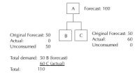
To understand two-level master scheduling, consider the following simple example in Figure 8-6. The bill of material structure illustrated shows an aggregate item, A, with components B and C, distributed at 50 percent each. A forecast for 100 A, therefore, generates a forecast for 50 each of B and C.
If A is a Planning Bill item, two-level scheduling is not supported, and the forecast is consumed only at the components, B and C. A Sales Order for 60 of item C will consume the entire forecast for C, actually overconsuming C's forecast. But the demand for B remains unchanged. Thus, if you were to run a plan with all the current demand data, the total demand is 110 units, even though the aggregate forecast was only 100.
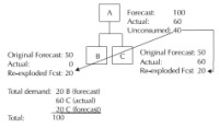
In the two-level scheduling scenario, the forecast is consumed at both the aggregate and the component levels. You can choose to re-explode the remaining aggregate forecast, with the results shown in Figure 8-7. Note that this will keep the aggregate demand constant, until the entire aggregate forecast is oversold. Notice, too, that this dynamically adjusts the mix of B and C, based on the forecast consumption.
The choice of forecast explosion methods is controlled by the explosion options used when you load the master schedule from a forecast. The Load/Copy/Merge Master Demand Schedule form lets you copy forecasts into your master schedule. Options let you choose whether to load the current (i.e. the remaining forecast, after consumption) or original forecast quantities, whether to explode the forecast, and whether to consume the forecast if consumption has not already occurred. If you explode the original quantities and select the Consume option, you will get the demand shown in Figure 8-6. If you explode the current quantities, you will get the demand picture that we've been calling two-level master scheduling (see Figure 8-7).
There are several potential pitfalls to be aware of in this process. If you explode original quantities, include sales orders, and do not select the consumption, you will inflate demand. The load process will do exactly what you ask -- it will explode the original quantities without consumption and add in sales orders that otherwise should have consumed that forecast. This will result in the very duplication of demand that forecast consumption is designed to prevent. (The load process does not allow you to consume if you are loading the current, i.e., already consumed, quantities.)
A second pitfall is loading a forecast that you have already exploded. This also results in duplicate demand -- you will load the existing forecast for the components or family members and then create additional forecast by exploding the family forecast.